For advanced users
For advanced users, we suggest you to start with HeLa_Noc.ipynb and Human_dev.ipynb. The following sections describe solutions for some special scenarios.
Handling stubborn clusters
If you find that the sequences in your data is hard to be separated. They are some options you can try:
For the input, try to combine other features, like secondary structures with the sequences. Or try to use sequences longer or shorter than 21-mers.
For
UMAP, increasingn_neighborsshould help to some extents.For
HDBSCAN, if you have been adjusting themin_samplesandmin_cluster_sizeparamters, you can also trycluster_selection_epsilonparameter. However, we suggest you to observe yourcondensed treeand determine if it is worth to continue.
Warning
The k-mers of your sequences should always be a ultra small fraction in the k-mers space.
Here is a breif example for Noc-treated HeLa cells:
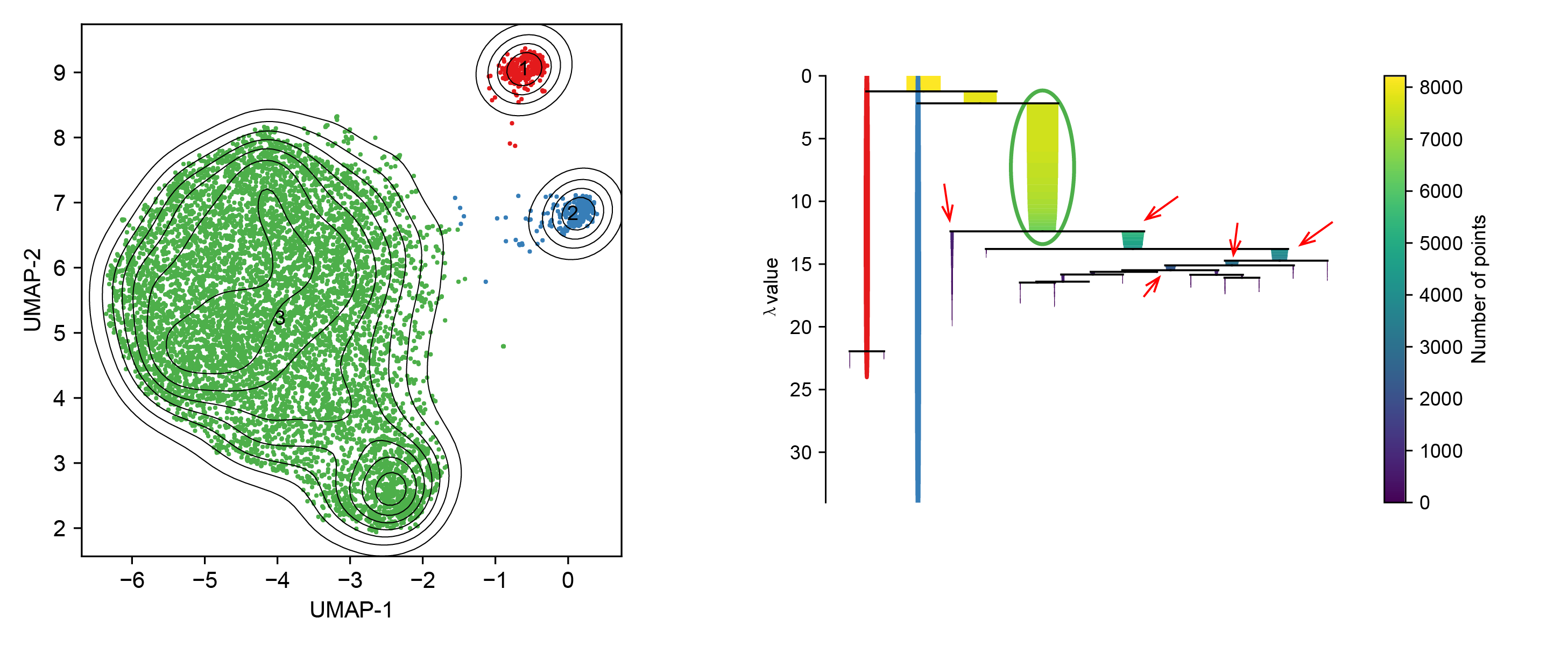
This one is the initial UMAP clusters we produced with eom function. We can clearly find that the clusters in red and blue are well clustered but the green one has two centroids. These two sub-clusters are two adjacent to each other and therefore considered to be one in HDBSCAN. It is exhausted to adjust the paramters to separate them without generating too many small clusters. So here we can be smart to use the leaf method for sub-clustering.
Now we have two choices, directly plot the leaves of all sites, or just plot the leaves for cluster #3. Here we use the latter strategy.

In this figure, we just keep cluster #1 and cluster #2 unchanged, but continue to split cluster #3. This generates the cluster #4 to #15, where #4 is what we want and #5 to #15 can be grouped into the orignally cluster #3. Then we have these beautiful clusters:

Tip
Saddly, HDBSCAN cannot use the lambda value to split the tree now.
Spike-in iMVP
Using “Spike-ins” (sequences with known modifications) is a quick way to find suitable clusters from the projections. Please read our RNA_seq_var.ipynb notebook for more information.
Phase matching
Owe to the position-sensitive feature of iMVP, we can have some interesting application.
In variant call from Nanopre RNA sequencing, an obvious problem is that the signal might not directly come from called base itself, but might come from its adjacent bases. Here, we call such phenomenon “phase mismatch”. In past, we might try to assign the signal of the variant to a selected adjacent base with some conditions. Now, with iMVP, we can have a more rational assignment because we now have the prior knowledge about the clusters. In our pratices, we first cluster the signals from xPore, and find that the first four clusters were from m6A signals in different phasese, while an additional one is in a m6Am-like motif. Here, we fix the phase of cluster #1 to #4 that assign the sequences without an “A” base centered to a specific downstream or upstream bases, by the pattern of the clusters. With such a method, we can correct the phases of the m6A and m6Am-like motifs.

Approximate clustering
When handling huge amount of sites, it is not easy for us to find a set of parameters perfectly clustering them. For most of the situations, like the global A-to-I RNA editing analysis, it is not necessary to assign very single point to a cluster. We want to have some snapshots. To solve this problem, we mimic the density profiling step in HDBSCAN to generate a histogram of site density first. With the density histogram, we can isolate the clusters with computer visulization methods (e.g., functions in openCV). In our practices, we first perform noise reduction to the histogram to filter out the low density connections between the clusters. Then we use find contours functions to link the connected pixels. We finally extract the clusters from the histogram and annotate them to the orignal sites. Read notebooks in RAPIDS folder for more information.
